Name: Sahil Shah UT EID: sbs2756
library(dplyr)##
## Attaching package: 'dplyr'## The following objects are masked from 'package:stats':
##
## filter, lag## The following objects are masked from 'package:base':
##
## intersect, setdiff, setequal, unionsetwd("/home/sahil/")
mlb <- read.csv("mlb.csv")
mlb <- mlb %>% subset(League!='Both')Summary of dataset The dataset that I have chosen to use contains the statistics of the top 100 batters in the MLB during the 2014 season. The variables in the dataset are AB which stands for at bat and means when a batter reaches a base via a hit, errror, or fielder’s choice, R which stands for run and means when a batter reaches home plate and scores a point for their team, H which stands for hit and means that the batter reached first base via only a hit, HR which stands for home run and represents the amount of times the batter has hit a home run, RBI which stands for run batted in and means that the batter allowed for runs to be scored when they batted, SB which stands for stolen base and represents the amount of bases the batter stole while a pitcher was throwing the ball, CS which stands for caught stealing and represents the number of times a batter was called out when trying to steal a base, AVG swhich stands for batting average and represents the the percentage in which the batter is able to hit the ball and make a play, OBP which stands for on base percentage and refers to how frequently a batter reaches base for each plate appearance, and SLG which stands for slugging percentage and refers to the amount of bases the batter gets per plate appearance.
#Conducting a MONOVA test
man <- manova(cbind(AB, R, H, HR, RBI, SB, CS, AVG, OBP, SLG)~League, data=mlb)
summary(man)
## Df Pillai approx F num Df den Df Pr(>F)
## League 1 0.13984 1.4144 10 87 0.1874
## Residuals 96summary.aov(man)## Response AB :
## Df Sum Sq Mean Sq F value Pr(>F)
## League 1 24137 24137.2 2.631 0.1081
## Residuals 96 880721 9174.2
##
## Response R :
## Df Sum Sq Mean Sq F value Pr(>F)
## League 1 476 476.08 1.3127 0.2548
## Residuals 96 34818 362.68
##
## Response H :
## Df Sum Sq Mean Sq F value Pr(>F)
## League 1 1592 1592.09 1.8622 0.1756
## Residuals 96 82077 854.97
##
## Response HR :
## Df Sum Sq Mean Sq F value Pr(>F)
## League 1 52.9 52.898 0.6202 0.4329
## Residuals 96 8187.9 85.291
##
## Response RBI :
## Df Sum Sq Mean Sq F value Pr(>F)
## League 1 684 684.50 1.3836 0.2424
## Residuals 96 47494 494.73
##
## Response SB :
## Df Sum Sq Mean Sq F value Pr(>F)
## League 1 75.5 75.469 0.6689 0.4155
## Residuals 96 10830.9 112.822
##
## Response CS :
## Df Sum Sq Mean Sq F value Pr(>F)
## League 1 2.61 2.6122 0.3428 0.5596
## Residuals 96 731.59 7.6207
##
## Response AVG :
## Df Sum Sq Mean Sq F value Pr(>F)
## League 1 0.000271 0.00027111 0.465 0.497
## Residuals 96 0.055978 0.00058310
##
## Response OBP :
## Df Sum Sq Mean Sq F value Pr(>F)
## League 1 0.002845 0.00284473 3.3563 0.07005 .
## Residuals 96 0.081367 0.00084757
## ---
## Signif. codes: 0 '***' 0.001 '**' 0.01 '*' 0.05 '.' 0.1 ' ' 1
##
## Response SLG :
## Df Sum Sq Mean Sq F value Pr(>F)
## League 1 0.00103 0.0010254 0.2863 0.5938
## Residuals 96 0.34380 0.00358130.05 / 1 #Bonferroni correction## [1] 0.05Discuss significant differences and if assumptions were met None of the numeric variables tested show a mean difference across the two leagues, American and National as none of the p-values calculated are below 0.05. Thus, I did not conduct any univariate ANOVA tests nor did I conduct any post-hoc t-tests. However, if a numeric variable was significant across the two leagues then I would have conducted these tests. Therefore, I onlt performed one test which was the MANOVA test and also had a p-value that was greater than 0..05 meaning that it was not significant. The probability I would have made a Type I error is 0.05 as that is the significance level that I was using to determine signifcance between the numeric variables and the two leagues. After conducting the Bonferroni correction, the significance level remained at 0.05 as the only test that I performed was the MANOVA so the level did not decrease. The assumptions for MANOVA were most likely not met as the numeric values for each player could be overdispersed with a wide range of percentages and amounts. However, if the manova test was significant then we would have to conduct 10 univariate ANOVA tests and 2 post hoc t tests for each one since there are two leagues in the MLB. Thus, the adjusted significance level would have been 0.05 / 31 = 0.0016.
#Randomization test - t-test
t.test(AVG~League, data=mlb)
##
## Welch Two Sample t-test
##
## data: AVG by League
## t = -0.68187, df = 95.144, p-value = 0.497
## alternative hypothesis: true difference in means is not equal to 0
## 95 percent confidence interval:
## -0.013011429 0.006358368
## sample estimates:
## mean in group American mean in group National
## 0.2800816 0.2834082#Null distribution
rand_dist <- vector()
for(i in 1:5000){
df <- data.frame(AVG=sample(mlb$AVG), League=mlb$League)
rand_dist[i] <- mean(df[df$League=='American',]$AVG) - mean(df[df$League=='National',]$AVG)
}
mlb%>%group_by(League)%>%summarize(s=mean(AVG))%>%summarize(diff(s))## # A tibble: 1 x 1
## `diff(s)`
## <dbl>
## 1 0.00333{hist(rand_dist); abline(v=c(-0.003326531 , 0.003326531), col='red')}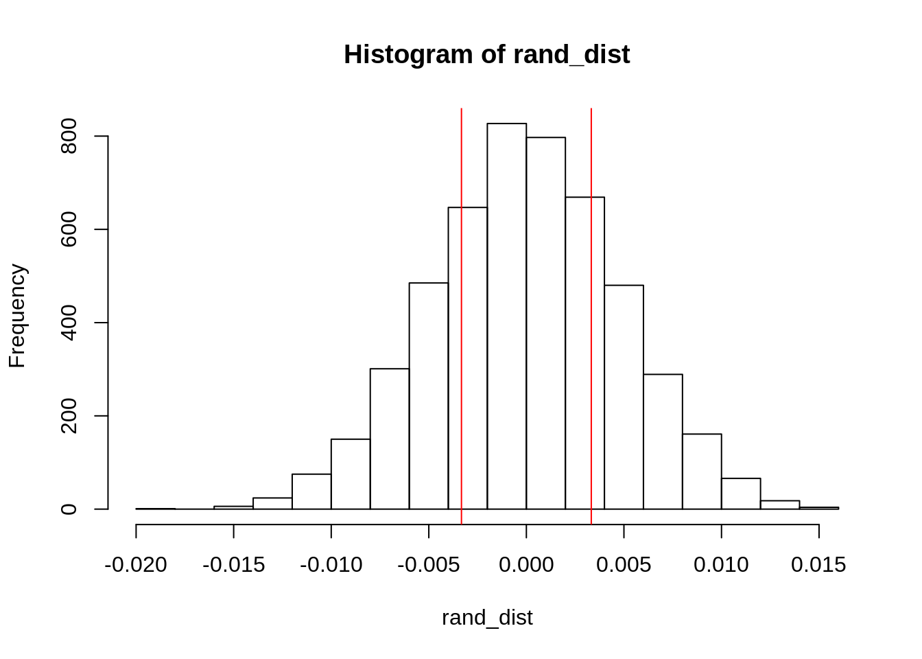
mean(rand_dist > 0.003326531)*2 #pvalue## [1] 0.4804State null and alternative hypotheses, perform the test, and interpret the results The null hypothesis is that there will be no difference in batting averages between the two leagues. The alternative hypothesis is that there is a difference in batting averages between the two leagues. When conducting a t-test, we can observe that the p-value calculated is greater than 0.05 meaning that the variable accounting for batting average is not significant. Thus, we fail to reject the null hypothesis and concude that there might not be a difference in batting averages between the two leagues.
#Linear regression model
library(ggplot2)
## Registered S3 methods overwritten by 'ggplot2':
## method from
## [.quosures rlang
## c.quosures rlang
## print.quosures rlanglibrary(tidyverse)## Registered S3 method overwritten by 'rvest':
## method from
## read_xml.response xml2## ── Attaching packages ─────────────────────────────────────────────────────────────────────────────────────────────────── tidyverse 1.2.1 ──## ✔ tibble 2.1.1 ✔ purrr 0.3.2
## ✔ tidyr 1.0.0 ✔ stringr 1.4.0
## ✔ readr 1.3.1 ✔ forcats 0.4.0## ── Conflicts ────────────────────────────────────────────────────────────────────────────────────────────────────── tidyverse_conflicts() ──
## ✖ dplyr::filter() masks stats::filter()
## ✖ dplyr::lag() masks stats::lag()library(lmtest)## Loading required package: zoo##
## Attaching package: 'zoo'## The following objects are masked from 'package:base':
##
## as.Date, as.Date.numericlibrary(sandwich)
new <- mlb
new$SLG <- new$SLG - mean(new$SLG)
new$AVG <- new$AVG - mean(new$AVG)
fit <- lm(new$AVG~new$SLG*new$League)
summary(fit)##
## Call:
## lm(formula = new$AVG ~ new$SLG * new$League)
##
## Residuals:
## Min 1Q Median 3Q Max
## -0.045010 -0.014776 -0.001833 0.012745 0.059973
##
## Coefficients:
## Estimate Std. Error t value Pr(>|t|)
## (Intercept) -0.001039 0.002964 -0.351 0.726643
## new$SLG 0.192951 0.048725 3.960 0.000146 ***
## new$LeagueNational 0.001946 0.004191 0.464 0.643479
## new$SLG:new$LeagueNational 0.040822 0.070752 0.577 0.565342
## ---
## Signif. codes: 0 '***' 0.001 '**' 0.01 '*' 0.05 '.' 0.1 ' ' 1
##
## Residual standard error: 0.02072 on 94 degrees of freedom
## Multiple R-squared: 0.2829, Adjusted R-squared: 0.26
## F-statistic: 12.36 on 3 and 94 DF, p-value: 6.947e-07coef(fit)## (Intercept) new$SLG
## -0.001039128 0.192950945
## new$LeagueNational new$SLG:new$LeagueNational
## 0.001946210 0.040821741new%>%ggplot(aes(x=SLG,y=AVG))+geom_point(aes(color=League))+geom_line(aes(y=predict(fit, new),color=League),size=1)+theme(legend.position=c(.9,.19))+ggtitle("t-test controlling for SLG")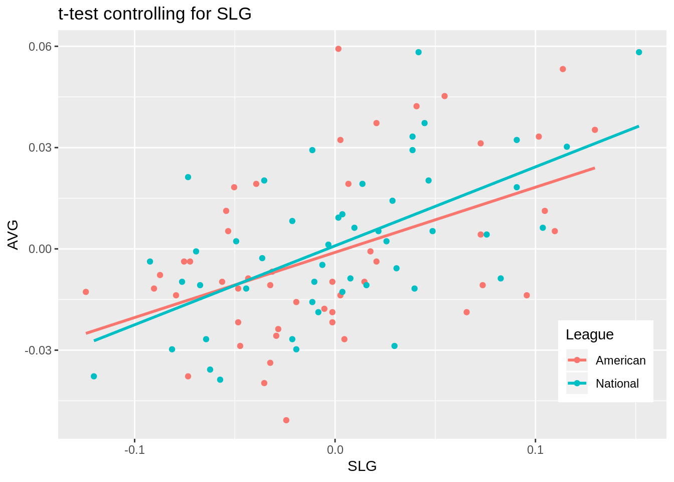
#Check linearity and homoskedstacity
resids<-fit$residuals
fitvals<-fit$fitted.values
ggplot()+geom_point(aes(fitvals,resids))+geom_hline(yintercept=0, color='red')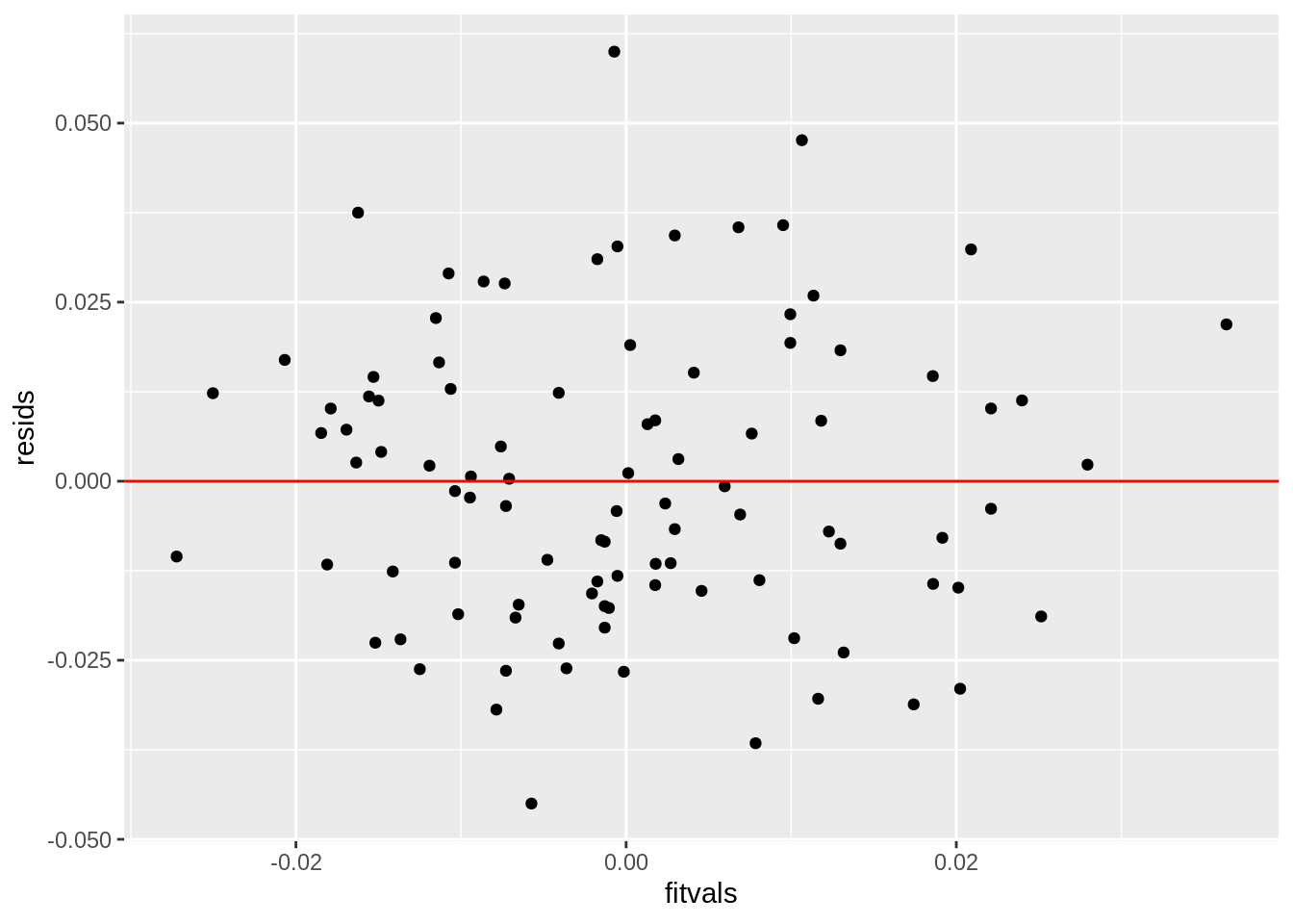
#Check normality
ggplot()+geom_qq(aes(sample=resids))+geom_qq_line(aes(sample=resids))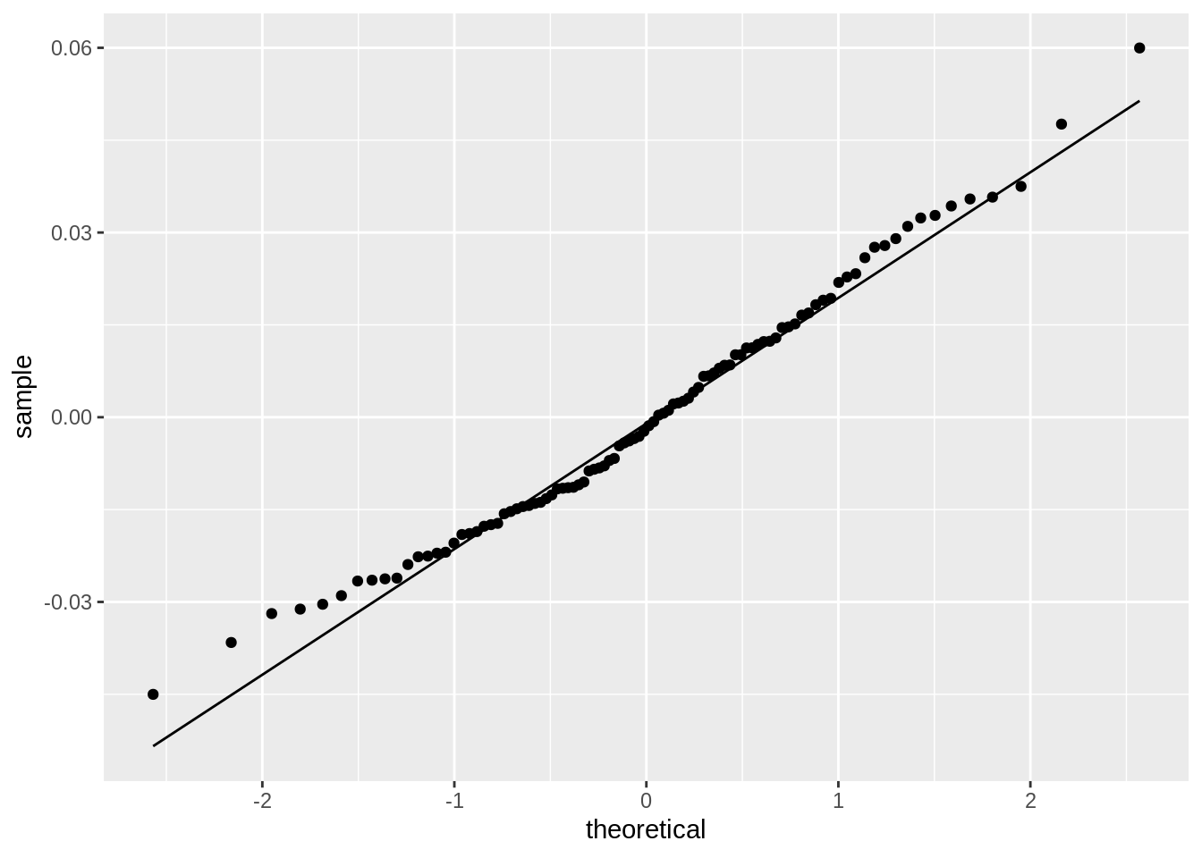
shapiro.test(resids) #Ho: distribution is normal##
## Shapiro-Wilk normality test
##
## data: resids
## W = 0.98481, p-value = 0.3212coeftest(fit, vcov=vcovHC(fit))##
## t test of coefficients:
##
## Estimate Std. Error t value Pr(>|t|)
## (Intercept) -0.0010391 0.0033182 -0.3132 0.7548512
## new$SLG 0.1929509 0.0481347 4.0086 0.0001223 ***
## new$LeagueNational 0.0019462 0.0042905 0.4536 0.6511543
## new$SLG:new$LeagueNational 0.0408217 0.0680631 0.5998 0.5501068
## ---
## Signif. codes: 0 '***' 0.001 '**' 0.01 '*' 0.05 '.' 0.1 ' ' 1no_int <- lm(new$AVG~new$SLG+new$League)
summary(no_int)##
## Call:
## lm(formula = new$AVG ~ new$SLG + new$League)
##
## Residuals:
## Min 1Q Median 3Q Max
## -0.044601 -0.014910 -0.001238 0.012912 0.059878
##
## Coefficients:
## Estimate Std. Error t value Pr(>|t|)
## (Intercept) -0.0009765 0.0029511 -0.331 0.741
## new$SLG 0.2123113 0.0352051 6.031 3.11e-08 ***
## new$LeagueNational 0.0019530 0.0041766 0.468 0.641
## ---
## Signif. codes: 0 '***' 0.001 '**' 0.01 '*' 0.05 '.' 0.1 ' ' 1
##
## Residual standard error: 0.02064 on 95 degrees of freedom
## Multiple R-squared: 0.2803, Adjusted R-squared: 0.2652
## F-statistic: 18.5 on 2 and 95 DF, p-value: 1.636e-07#Proportion of variance
0.048725+0.004191+0.070752## [1] 0.123668Interpret the coefficient estimates, Check assumptions, Discuss significance of results, including any changes from before/after robust SEs if applicable, What proportion of the variation in the outcome does your model explain The coefficient estimates for SLG, being in the National league, and the interaction between the two variables are as follows: 0.192950945, 0.001946210, 0.040821741. This means that for every unit increase in SLG, slugging percentage, a player’s batting average will increase by 0.192950945; if a player is in the National league then that player’s batting average increases by 0.001946210 compared to being in the American league; and if a plyer is in the National league and for every unit increase in the player’s SLG statistic, their batting average increases by 0.040821741. All assumptions of linearity, homoskedstacity, and normality have all been met. This is determined by the graphs produced above and normality was further proven true by conducting a a Shapiro-Wilkes test as obtaining a p-value greater than 0.05 confirming that normality has been met. After recomputing the regression results with robust standard errors, the only variable that was significant was SLG, a player’s slugging percentage. However, previously, the SLG statistic was significant before recomputing the regression results as it had a p-value of 0.000146 and a p-value of 0.0001223 after recomputing. However, all the standard error values for each variable changed as the values before, for SLG, being in the National league, and their interaction, were 0.048725, 0.004191, and 0.070752, respectively. After recomputing the standard error values for SLG, being in the National league, and their interaction were 0.0481347, 0.0042905, and 0.0680631, respecitvely. If the amount of variance that each variable explained were added together, the total amount of variance explained by the model would be 0.123668.
#Bootstrapped SE's
set.seed(12)
samp_distn<-replicate(5000, {
boot_dat<-new[sample(nrow(new),replace=TRUE),]
fit1<-lm(AVG~SLG*League,data=boot_dat)
coef(fit1)
})
## Estimated SEs
samp_distn%>%t%>%as.data.frame%>%summarize_all(sd)
## (Intercept) SLG LeagueNational SLG:LeagueNational
## 1 0.003311479 0.04708495 0.00423657 0.06655386Discuss any changes you observe in SEs and p-values using these SEs compared to the original SEs and the robust SEs Although there are slight differences between the bootstrapped standard error values and the original and robust standard error values, the differences are miniscule. The standard error value from the bootstrapped model for SLG, being in the National league and their interaction were 0.0472222, 0.004225108, and 0.06487124, respecitvely, whereas the standard error value found in the original model for the same variables were 0.048725, 0.004191, and 0.070752, respecitvely. This means that the bootstrapping technique is an accurate method in trying to determine the significance of variables in a linear model. The p-values are also similar in that only the SLG variable is significant in the model whereas the other two are not.
library(plotROC)
#Logistic regression
class_diag<-function(probs,truth){

  tab<-table(factor(probs>.5,levels=c("FALSE","TRUE")),truth)
  acc=sum(diag(tab))/sum(tab)
  sens=tab[2,2]/colSums(tab)[2]
  spec=tab[1,1]/colSums(tab)[1]
  ppv=tab[2,2]/rowSums(tab)[2]

  if(is.numeric(truth)==FALSE & is.logical(truth)==FALSE) truth<-as.numeric(truth)-1

  #CALCULATE EXACT AUC
  ord<-order(probs, decreasing=TRUE)
  probs <- probs[ord]; truth <- truth[ord]

  TPR=cumsum(truth)/max(1,sum(truth))
  FPR=cumsum(!truth)/max(1,sum(!truth))

  dup<-c(probs[-1]>=probs[-length(probs)], FALSE)
  TPR<-c(0,TPR[!dup],1); FPR<-c(0,FPR[!dup],1)

  n <- length(TPR)
  auc<- sum( ((TPR[-1]+TPR[-n])/2) * (FPR[-1]-FPR[-n]) )

  data.frame(acc,sens,spec,ppv,auc)
}
log_fit <- glm(League~AVG+SLG+HR+SB+OBP, data=mlb, family='binomial')
summary(log_fit)
##
## Call:
## glm(formula = League ~ AVG + SLG + HR + SB + OBP, family = "binomial",
## data = mlb)
##
## Deviance Residuals:
## Min 1Q Median 3Q Max
## -1.67872 -1.11054 -0.02849 1.13175 1.69285
##
## Coefficients:
## Estimate Std. Error z value Pr(>|z|)
## (Intercept) -3.25102 2.84902 -1.141 0.2538
## AVG -23.27013 16.59576 -1.402 0.1609
## SLG 11.67240 9.51595 1.227 0.2200
## HR -0.09304 0.05025 -1.852 0.0641 .
## SB -0.01401 0.02162 -0.648 0.5171
## OBP 18.04861 10.25840 1.759 0.0785 .
## ---
## Signif. codes: 0 '***' 0.001 '**' 0.01 '*' 0.05 '.' 0.1 ' ' 1
##
## (Dispersion parameter for binomial family taken to be 1)
##
## Null deviance: 135.86 on 97 degrees of freedom
## Residual deviance: 127.54 on 92 degrees of freedom
## AIC: 139.54
##
## Number of Fisher Scoring iterations: 4prob <- predict(log_fit, type='response')
class_diag(prob, mlb$League)## acc sens spec ppv auc
## Both 0.3061224 NaN 0.6122449 0 0.6522282#Confusion matrix
table(predict=as.numeric(prob>.5),truth=mlb$League)%>%addmargins## truth
## predict American Both National Sum
## 0 30 0 21 51
## 1 19 0 28 47
## Sum 49 0 49 98#Density plot
mlb$logit<-predict(log_fit,type="link")
mlb$League <- as.factor(mlb$League)
mlb%>%ggplot()+geom_density(aes(logit,color=League,fill=League),alpha=.4)+theme(legend.position=c(.85,.85))+ geom_vline(xintercept=0)+xlab("predictor (logit)")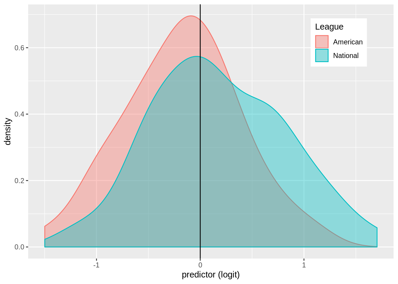
#ROC and AUC
mlb$League <- ifelse(mlb$League=='National', 1, 0)
classify <- mlb %>% transmute(prob=predict(log_fit, type='response') , truth=League)
ROCplot <- ggplot(classify) + geom_roc(aes(d=truth, m=prob), n.cuts=0)
ROCplot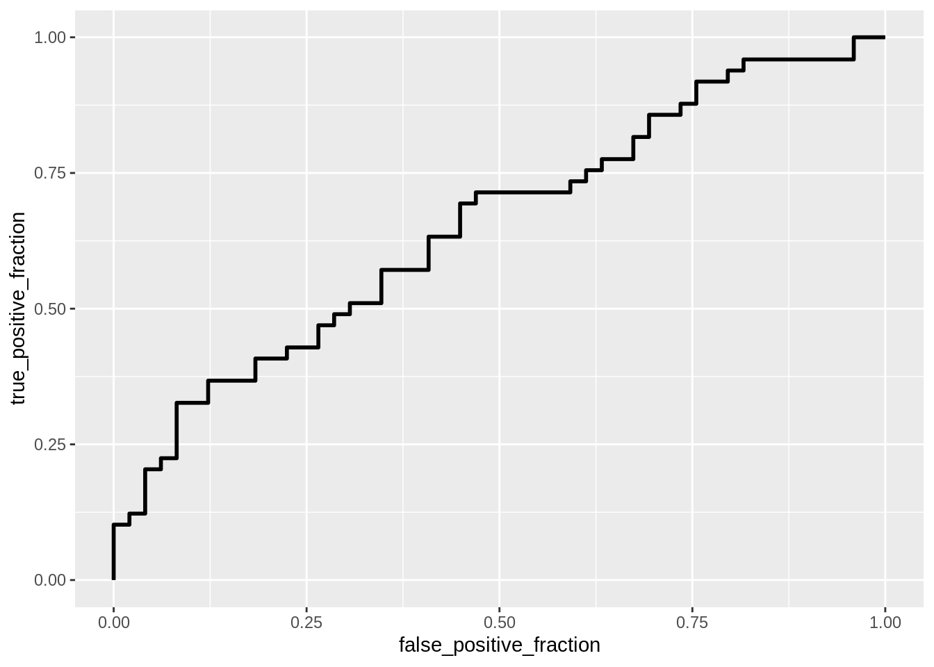
calc_auc(ROCplot)## PANEL group AUC
## 1 1 -1 0.6522282#10-fold
set.seed(1234)
k=10
data1<-mlb[sample(nrow(mlb)),] #put dataset in random order
folds<-cut(seq(1:nrow(mlb)),breaks=k,labels=F) #create folds
diags<-NULL
for(i in 1:k){ # FOR EACH OF 10 FOLDS
train<-data1[folds!=i,] #CREATE TRAINING SET
test<-data1[folds==i,] #CREATE TESTING SET
truth<-test$League
log_fit2<- glm(League~AVG+SLG+HR+SB+OBP, data=train, family='binomial')
probs<- predict(log_fit2, newdata=test, type='response')
diags<-rbind(diags,class_diag(probs,truth))
}
apply(diags,2,mean) #AVERAGE THE DIAGNOSTICS ACROSS THE 10 FOLDS## acc sens spec ppv auc
## 0.5088889 0.4985714 0.5592857 0.5228571 0.5949246Interpret coefficient estimates in context, discuss the Accuracy, Sensitivity (TPR), Specificity (TNR), and Recall (PPV) of your model, interpret ROC and AUC, and report average out-of-sample Accuracy, Sensitivity, and Recall The coefficient estimates calculated for each variable from AVG, SLG, HR, SB, and OBP are as follows: -23.27013, 11.67240, -0.09304, -0.01401, and 18.04861. For the AVG variable this means that for every unit increase in batting average, the likelihood that a player is in the National league decreases by 23.27013 units. For the SLG variable this means that for every unit increse in slugging percentage, the likelihood that a player is in the National league increases by 11.67240 units. For the HR variable this means that for every home run hit, the likelihood that a player plays in the National league decreases by 0.09304 units. For the SB variable this means that for every stolen base, the likelihood that a player plays in the National league decreases by 0.01401 units. For the OBP variable this means that for every unit increse in on base percentage, the likelihood a player plays in the National league increases by 18.04861 units. The accuracy, sensitivity, specificity, and recall values found are 0.5918367, 0.5714286, 0.6122449, and 0.5957447, respectively. These values mean that the model created is an alright model for predicting which player will be in the National or American league based in their AVG, SLG, HR, SB, and OBP statistics. However, the accuracy of the model is only about 60% which means that more variables may need to be added into the model to find a better predictor of determining which player would play in each league. The sensitivity and specificity are also around 60% which means that the model correctly predicts a positive and a negative only about 60% of the time. Furthermore, the recall value is also around 60% which means that the model correctly classifies the results only about 60% of the time as well. The assertion that this model is not a great predictor in classifying which player plays in a certain league is further confirmed when analyzing the ROC curve. The ROC plot shows us that there may be certain instances where the model predicts incorrectly and only predicts the data correctly a little over 50% of the time which is consistent with the classification data we previously analyzed. The AUC value found was 0.6522282 which means that the probability of randomly selecting a person that plays in the National league has a higher prediction that a randomly selected person that plays in the American league. The average out-of-sample accuracy, sensitivity, and recall values found were 0.5444444, 0.5659524, and 0.6178571, respectively.
#LASSO
library(glmnet)
## Loading required package: Matrix##
## Attaching package: 'Matrix'## The following objects are masked from 'package:tidyr':
##
## expand, pack, unpack## Loading required package: foreach##
## Attaching package: 'foreach'## The following objects are masked from 'package:purrr':
##
## accumulate, when## Loaded glmnet 2.0-16y<-as.matrix(mlb$League) ###save response variable
x<-model.matrix(log_fit) ###save matrix of all predictors (dropping the response variable)
x <- x[,-1]
cv<-cv.glmnet(x,y,family="binomial")
lasso<-glmnet(x,y,family="binomial",lambda=cv$lambda.1se)
coef(lasso)## 6 x 1 sparse Matrix of class "dgCMatrix"
## s0
## (Intercept) -3.469447e-17
## AVG 0.000000e+00
## SLG .
## HR .
## SB .
## OBP .fit<- glm(League~AVG+SLG+HR+SB+OBP, data=mlb, family='binomial')
prob <- predict(fit, type='response')
class_diag(prob, mlb$League)## acc sens spec ppv auc
## 1 0.5918367 0.5714286 0.6122449 0.5957447 0.6522282set.seed(1245)
k=10
# your code here
data1<-mlb[sample(nrow(mlb)),] #put dataset in random order
folds<-cut(seq(1:nrow(mlb)),breaks=k,labels=F) #create folds
diags<-NULL
for(i in 1:k){ # FOR EACH OF 10 FOLDS
train<-data1[folds!=i,] #CREATE TRAINING SET
test<-data1[folds==i,] #CREATE TESTING SET
truth<-test$League
lasso_fit<- glm(League~AVG+SLG+HR+SB+OBP, data=train, family='binomial')
probs<- predict(lasso_fit, newdata=test, type='response')
diags<-rbind(diags,class_diag(probs,truth))
}
apply(diags,2,mean) #AVERAGE THE DIAGNOSTICS ACROSS THE 10 FOLDS## acc sens spec ppv auc
## 0.4900000 0.5141667 0.4750000 0.5163492 0.5728889Discuss which variables are retained, compare model’s out-of-sample accuracy to that of your logistic regression in part 5 The only variable that was retained after running a LASSO regression was the AVG variable. The out-of-sample accuracy value found was 0.5322222 is similar to, but less than the one found in the logisitc regression in part 5, 0.5918367. However, the value is more similar to the out-of-sample accuracy value found in part 5, 0.5444444.