#Joining dataframes
demo <- as.data.frame(MplsDemo)
stops <- as.data.frame(MplsStops)
stops <- stops %>% pivot_wider(names_from=problem, values_from=preRace)
stops <- stops %>% pivot_longer(cols=c('suspicious', 'traffic'), names_to='problem', values_to='preRace')
fulldata <- right_join(demo, stops) %>% na.omit(col=personSearch)
## Joining, by = "neighborhood"## Warning: Column `neighborhood` joining character vector and factor, coercing
## into character vectordiff_neighborhoods <- anti_join(demo, stops)## Joining, by = "neighborhood"## Warning: Column `neighborhood` joining character vector and factor, coercing
## into character vector#Adding variables in the joined dataframe
fulldata <- fulldata %>% mutate(white_pop=white*population, black_pop=black*population, foreign_pop=foreignBorn*population, in_poverty=poverty*population, college_educated=collegeGrad*population)
fulldata <- fulldata %>% group_by(neighborhood, race) %>% mutate(race_number_of_stops=n())
fulldata <- fulldata %>% group_by(neighborhood, gender) %>% mutate(gender_number_of_stops=n())The reason I decided to do a right join on the two data frames is because this would provide information about each person and the neighborhood they live in to determine if certain precincts have more arrests in one neighborhood over another and if there is a disproporionate number of arrests based on race or gender. Also, no cases in the MplsStops nor the MplsDemo datasets were dorpped when joined together.
#Shows number of arrests by race
race_stops <- fulldata %>% group_by(race) %>% summarize(sum_stops=sum(race_number_of_stops)) %>% arrange(sum_stops)
glimpse(race_stops)
## Observations: 8
## Variables: 2
## $ race <fct> Asian, Other, Latino, Native American, East African, Unknow…
## $ sum_stops <int> 2330, 9270, 16587, 31967, 35931, 394986, 670303, 1670265#Shows number of arrests by gender
gender_stops <- fulldata %>% group_by(gender) %>% summarize(sum_stops=sum(gender_number_of_stops))
glimpse(gender_stops)## Observations: 3
## Variables: 2
## $ gender <fct> Female, Male, Unknown
## $ sum_stops <int> 431936, 3735595, 188708#Shows number of arrests by gender
gender_stops <- fulldata %>% group_by(gender) %>% summarize(sum_stops=sum(gender_number_of_stops))
glimpse(gender_stops)## Observations: 3
## Variables: 2
## $ gender <fct> Female, Male, Unknown
## $ sum_stops <int> 431936, 3735595, 188708#Number of stops by neighborhood
fulldata %>% select(race, neighborhood, race_number_of_stops) %>% group_by(neighborhood) %>% summarize(sum_stops=sum(race_number_of_stops)) %>% arrange(desc(sum_stops))## Adding missing grouping variables: `gender`## # A tibble: 84 x 2
## neighborhood sum_stops
## <chr> <int>
## 1 Downtown West 673248
## 2 Jordan 329931
## 3 Hawthorne 301478
## 4 Whittier 222570
## 5 Nicollet Island - East Bank 133144
## 6 Folwell 113918
## 7 Lyndale 109205
## 8 Marcy Holmes 91645
## 9 Willard - Hay 91184
## 10 Lowry Hill East 79067
## # … with 74 more rowsfulldata %>% select(neighborhood, white, black, foreignBorn) %>% subset(select=-gender) %>% unique() %>% arrange(desc(black))## Adding missing grouping variables: `gender`## # A tibble: 84 x 4
## neighborhood white black foreignBorn
## <chr> <dbl> <dbl> <dbl>
## 1 Sumner - Glenwood 0.087 0.656 0.292
## 2 Phillips West 0.199 0.538 0.318
## 3 Willard - Hay 0.215 0.516 0.141
## 4 Cedar Riverside 0.353 0.464 0.408
## 5 Hawthorne 0.186 0.456 0.167
## 6 Jordan 0.183 0.453 0.155
## 7 Harrison 0.31 0.427 0.163
## 8 Ventura Village 0.214 0.424 0.329
## 9 McKinley 0.22 0.416 0.161
## 10 Folwell 0.285 0.403 0.116
## # … with 74 more rows#Ratio of blacks to whites in each neighborhood
fulldata %>% mutate(bw=black_pop/white_pop) %>% select(neighborhood, bw) %>% subset(select=-gender) %>% unique() %>% arrange(desc(bw))## Adding missing grouping variables: `gender`## # A tibble: 84 x 2
## neighborhood bw
## <chr> <dbl>
## 1 Sumner - Glenwood 7.54
## 2 Phillips West 2.70
## 3 Jordan 2.48
## 4 Hawthorne 2.45
## 5 Willard - Hay 2.4
## 6 Ventura Village 1.98
## 7 McKinley 1.89
## 8 East Phillips 1.83
## 9 Folwell 1.41
## 10 Harrison 1.38
## # … with 74 more rows#Ratio of non-white neighborhoods
non_white_neigh <- fulldata %>% mutate(ratio=(black_pop+foreign_pop)/white_pop) %>% select(neighborhood, ratio) %>% subset(select=-gender) %>% unique() %>% arrange(desc(ratio))## Adding missing grouping variables: `gender`glimpse(non_white_neigh)## Observations: 84
## Variables: 2
## $ neighborhood <chr> "Sumner - Glenwood", "East Phillips", "Phillips West", "…
## $ ratio <dbl> 10.8965517, 4.3464052, 4.3015075, 3.5186916, 3.3494624, …#Number of citations by race
race_cites <- fulldata %>% select(race, citationIssued) %>% filter(citationIssued=='YES') %>% group_by(race) %>% summarise(sum_cites=n())## Adding missing grouping variables: `neighborhood`, `gender`glimpse(race_cites)## Observations: 8
## Variables: 2
## $ race <fct> Black, White, Unknown, East African, Latino, Native America…
## $ sum_cites <int> 1383, 907, 187, 134, 198, 84, 79, 54#Gives ratio of citations per stop by each race
race_cites_per_stop <- full_join(race_stops, race_cites) %>% mutate(perc_of_cites=100*(sum_cites/sum_stops))## Joining, by = "race"glimpse(race_cites_per_stop)## Observations: 8
## Variables: 4
## $ race <fct> Asian, Other, Latino, Native American, East African, Un…
## $ sum_stops <int> 2330, 9270, 16587, 31967, 35931, 394986, 670303, 1670265
## $ sum_cites <int> 54, 79, 198, 84, 134, 187, 907, 1383
## $ perc_of_cites <dbl> 2.31759657, 0.85221143, 1.19370591, 0.26277098, 0.37293…#Gives ratio of citations per stop by gender
gender_cites <- fulldata %>% select(gender, citationIssued) %>% filter(citationIssued=='YES') %>% group_by(gender) %>% summarise(sum_cites=n())## Adding missing grouping variables: `neighborhood`full_join(gender_stops, gender_cites) %>% mutate(perc_of_cites=100*(sum_cites/sum_stops))## Joining, by = "gender"## # A tibble: 3 x 4
## gender sum_stops sum_cites perc_of_cites
## <fct> <int> <int> <dbl>
## 1 Female 431936 791 0.183
## 2 Male 3735595 2071 0.0554
## 3 Unknown 188708 164 0.0869#College educated in each neighborhood - 7 out of the top 10 non-white neighborhoods are the least college educated in Minneapolis
college_edu <- fulldata %>% select(neighborhood, collegeGrad) %>% subset(select=-gender) %>% unique() %>% arrange(collegeGrad)## Adding missing grouping variables: `gender`glimpse(college_edu)## Observations: 84
## Variables: 2
## $ neighborhood <chr> "McKinley", "Jordan", "Hawthorne", "Sumner - Glenwood", …
## $ collegeGrad <dbl> 0.122, 0.142, 0.151, 0.165, 0.173, 0.181, 0.196, 0.203, …#Summary stats for each race
race_stops_summary <- fulldata %>% group_by(race) %>% summarize(mean_stops=mean(race_number_of_stops), sd_stops=sd(race_number_of_stops), var_stops=var(race_number_of_stops)) %>% arrange(mean_stops)
glimpse(race_stops_summary)## Observations: 8
## Variables: 4
## $ race <fct> Asian, Other, Latino, East African, Native American, Unkno…
## $ mean_stops <dbl> 9.708333, 16.916058, 23.133891, 44.414091, 47.079529, 88.2…
## $ sd_stops <dbl> 7.465285, 12.604527, 16.884886, 41.967548, 38.546293, 52.7…
## $ var_stops <dbl> 55.73047, 158.87411, 285.09937, 1761.27510, 1485.81667, 27…quantile(fulldata$race_number_of_stops)## 0% 25% 50% 75% 100%
## 1 37 93 186 726min(fulldata$race_number_of_stops)## [1] 1max(fulldata$race_number_of_stops)## [1] 726#Summary statistice for each gender
gender_stops_summary <- fulldata %>% group_by(gender) %>% summarize(mean_stops=mean(gender_number_of_stops), sd_stops=sd(gender_number_of_stops), var_stops=var(gender_number_of_stops)) %>% arrange(mean_stops)
glimpse(gender_stops_summary)## Observations: 3
## Variables: 4
## $ gender <fct> Unknown, Female, Male
## $ mean_stops <dbl> 62.77711, 109.29555, 331.84641
## $ sd_stops <dbl> 39.16807, 74.74386, 277.02384
## $ var_stops <dbl> 1534.137, 5586.644, 76742.206quantile(fulldata$gender_number_of_stops)## 0% 25% 50% 75% 100%
## 1 68 150 316 1014min(fulldata$gender_number_of_stops)## [1] 1max(fulldata$gender_number_of_stops)## [1] 1014#Number of stops per precinct
pol_prec_demo <- fulldata %>% select(policePrecinct, white, black, foreignBorn) %>% subset(select=-c(neighborhood, gender)) %>% unique() %>% mutate(perc_foreign=100*foreignBorn)## Adding missing grouping variables: `neighborhood`, `gender`nstops_precinct <- fulldata %>% group_by(policePrecinct) %>% summarize(sum_stops=n())
avg_foreign_born <- pol_prec_demo %>% group_by(policePrecinct) %>% summarize(mean_foreign=mean(foreignBorn))
full_join(avg_foreign_born, nstops_precinct) %>% arrange(mean_foreign)## Joining, by = "policePrecinct"## # A tibble: 5 x 3
## policePrecinct mean_foreign sum_stops
## <int> <dbl> <int>
## 1 5 0.101 4359
## 2 4 0.136 4082
## 3 2 0.150 3311
## 4 3 0.151 3929
## 5 1 0.225 2534Each of the functions used thus far were to find correlations between certain variables and determine if we can observe a pattern between the numeric variables. Each function used was necessary in tring to interpret certain correlations that could be portrayed in plots for the next portion of this project.
#Create graphs
#College educated by race
white_college <- fulldata %>% ggplot(aes(x=white, y=collegeGrad)) + geom_line(stat='identity') + ylab('College Educated') + xlab('Percent White in Neighborhood')
black_college <- fulldata %>% ggplot(aes(x=black, y=collegeGrad)) + geom_line(stat='identity') + ylab('College Educated') + xlab('Percent Black in Neighborhood')
college_income <- fulldata %>% ggplot(aes(x=collegeGrad, y=hhIncome)) + geom_line(stat='identity') + ylab('Household Income') + xlab('Percent Foreign Born in Neighborhood')
grid.arrange(white_college, black_college, college_income)
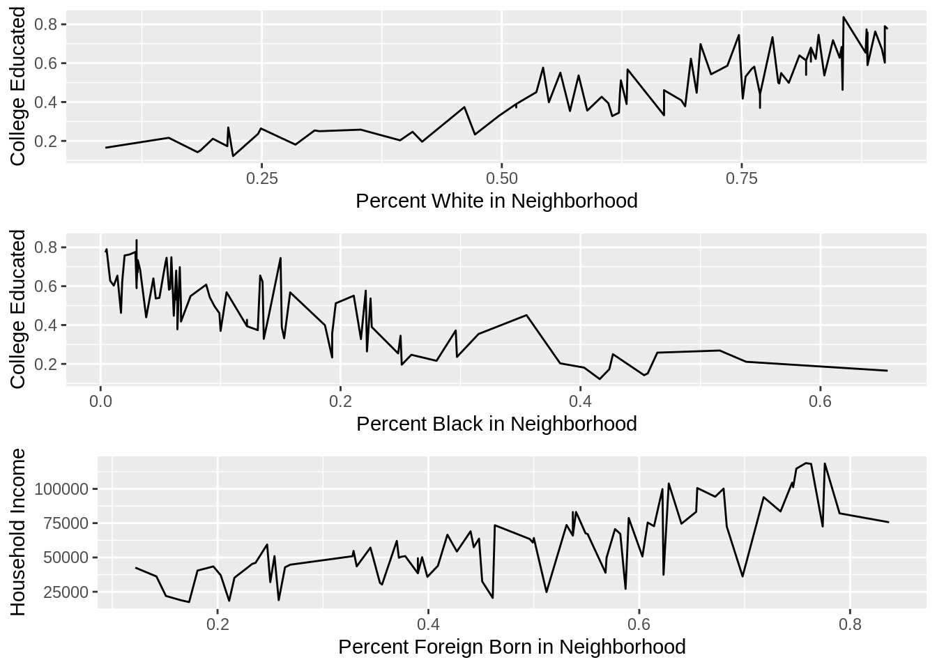
These three graphs portray the relationship between college education, race, and household income and were necessary to show how college education disproportionately favors those that are white compared to those that are black. We can observe from these plots that neighborhoods that have a higher population of whites tend to be college educated and those that are colege educated have higher household incomes. Thus, we can interpret that whites have higher household incomes and that neighborhoods that are predominantly white are disproportionately richer than their non-white counterparts.
#Number of stops by race
nstops_bar <- race_stops %>% ggplot(aes(x=race, y=sum_stops, fill=race)) + geom_bar(stat='identity') + xlab('Race') + ylab('Number of Stops')
ncites_bar <- race_cites_per_stop %>% ggplot(aes(x=race, y=perc_of_cites, fill=race)) + geom_bar(stat='identity') + xlab('Race') + ylab('Percent Chance of a Citation per Stop')
grid.arrange(nstops_bar, ncites_bar)
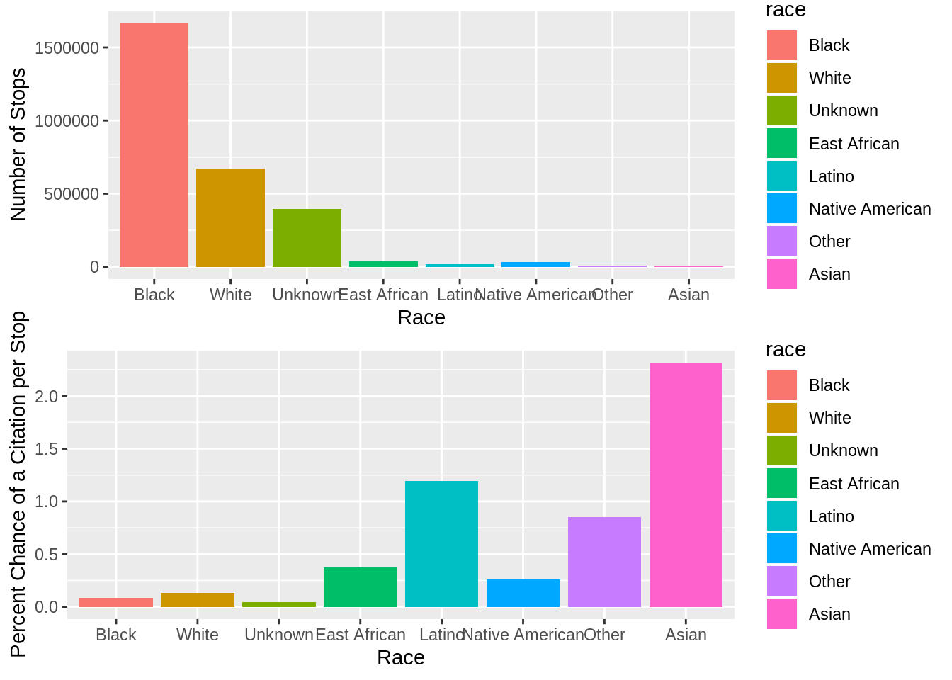
These two bar graphs display data related to the number of stops by race and the percent chance that a certain race will be issued a citation when stopped. Interestingly, although blacks are stopped at a disproportionately high rate, asians and latinos are issued the most citations. Thus, this information shows that even if a certain race is stopped at a high rate that does not necessarily mean that they will receive a citation of any sort as asians and latinos are stopped at a relatively low rate. Although there are some that were of an unknown race and were stopped that could potentially skew the data, there are enough data points in order to make certain conclusions.
#Relationship between foreign born and number of stops per precinct
foreign_stops_bar <- pol_prec_demo %>% ggplot(aes(x=policePrecinct, y=perc_foreign, fill=policePrecinct)) + geom_bar(stat='summary', fun.y='mean') + xlab('Police Precinct') + ylab('Average Percent of Foreigners per Precinct')
precinct_nstops <- nstops_precinct %>% ggplot(aes(x=policePrecinct, y=sum_stops, fill=policePrecinct)) + geom_bar(stat='identity') + xlab('Police Precinct') + ylab('Total Number of Stops per Precinct')
grid.arrange(precinct_nstops, foreign_stops_bar)
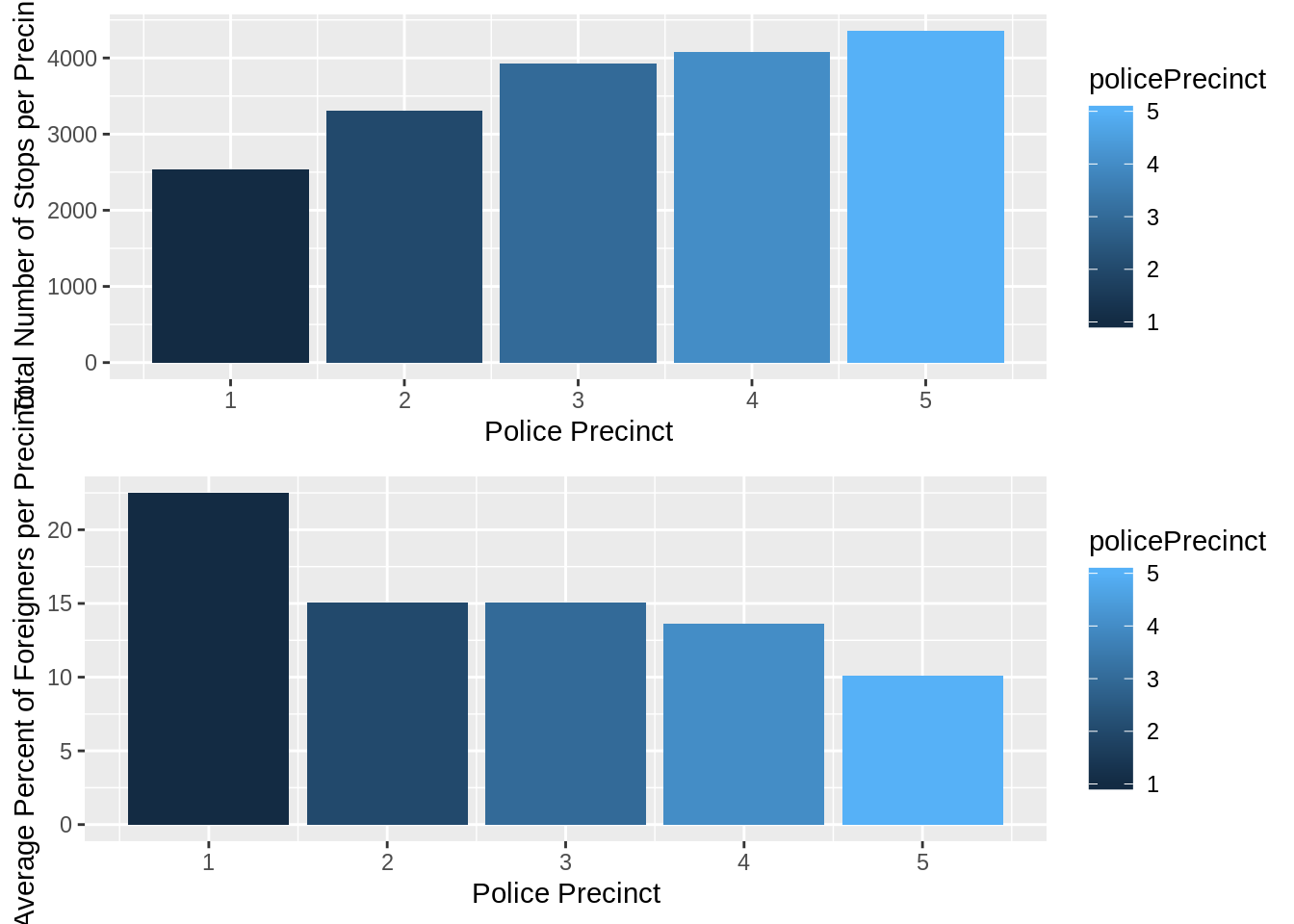
These two bar graphs display an interesting trend within the number of stops each police precinct makes. When looking at the first graph, one can determine the average number of stops each precinct has made. The second graph tells us the average number of foreigners contained within eahc precinct’s jurisdiction. When comparing the two graphs, it is apparent that precincts with more foreigners within their jurisdiction have less stops. However, when exploring the dataset from before, we could determine that blacks and whites were both arrested at high rates within each precinct and no trand could be found from that data. Thus, we can conclude that neighborhoods with more foreign born residents will have less stops in their area.
#PCA
#A variable is created to view the correlation matrix of the numeric variables
full <- fulldata %>% select(white, black, foreignBorn, hhIncome, race_number_of_stops, collegeGrad, gender_number_of_stops) %>% subset(select=-c(neighborhood, gender)) %>% unique()
## Adding missing grouping variables: `neighborhood`, `gender`cor_mat <- full %>% cor()
cor_mat## white black foreignBorn hhIncome
## white 1.0000000 -0.9088666 -0.7211797 0.6945528
## black -0.9088666 1.0000000 0.5951981 -0.6608667
## foreignBorn -0.7211797 0.5951981 1.0000000 -0.6385357
## hhIncome 0.6945528 -0.6608667 -0.6385357 1.0000000
## race_number_of_stops -0.2221233 0.1951111 0.1841638 -0.1636191
## collegeGrad 0.8795814 -0.7962216 -0.5759628 0.7389111
## gender_number_of_stops -0.3014754 0.2538835 0.2746756 -0.2402555
## race_number_of_stops collegeGrad gender_number_of_stops
## white -0.2221233 0.8795814 -0.3014754
## black 0.1951111 -0.7962216 0.2538835
## foreignBorn 0.1841638 -0.5759628 0.2746756
## hhIncome -0.1636191 0.7389111 -0.2402555
## race_number_of_stops 1.0000000 -0.1446711 0.3359812
## collegeGrad -0.1446711 1.0000000 -0.1911664
## gender_number_of_stops 0.3359812 -0.1911664 1.0000000#A variable is created to be used for principle component analysis as rotations are given by using the function, prcomp()
full_pca <- fulldata %>% select(white, black, foreignBorn, hhIncome, race_number_of_stops, collegeGrad, gender_number_of_stops) %>% subset(select=-c(neighborhood, gender)) %>% unique() %>% scale() %>% prcomp()## Adding missing grouping variables: `neighborhood`, `gender`#These were to show the statistics of the principal component analysis before plotting
full_pca$rotation## PC1 PC2 PC3 PC4
## white -0.4726675 0.08594555 -0.03203439 0.18357023
## black 0.4442097 -0.11082752 0.07174391 -0.37659841
## foreignBorn 0.3916580 -0.02340632 -0.11530995 0.79314070
## hhIncome -0.4128878 0.11401364 0.01739029 -0.25706154
## race_number_of_stops 0.1497552 0.71306574 0.68142345 0.05488754
## collegeGrad -0.4419161 0.19569913 -0.09390972 0.31233433
## gender_number_of_stops 0.1940987 0.64809163 -0.71208907 -0.16958014
## PC5 PC6 PC7
## white -0.29891217 -0.08026881 -0.79917644
## black 0.27988737 -0.63322345 -0.40510807
## foreignBorn 0.39104784 0.09702222 -0.20336137
## hhIncome 0.80614759 0.28706980 -0.13363553
## race_number_of_stops -0.03181054 0.02153920 -0.01685888
## collegeGrad 0.16013386 -0.70589665 0.36892728
## gender_number_of_stops -0.05354873 0.04481730 -0.03998260full_pca %>% summary()## Importance of components:
## PC1 PC2 PC3 PC4 PC5 PC6 PC7
## Standard deviation 2.0187 1.0846 0.81516 0.69616 0.61030 0.42543 0.21471
## Proportion of Variance 0.5821 0.1681 0.09493 0.06923 0.05321 0.02586 0.00659
## Cumulative Proportion 0.5821 0.7502 0.84512 0.91435 0.96756 0.99341 1.00000cor_mat %>% eigen()## eigen() decomposition
## $values
## [1] 4.07496678 1.17635824 0.66448143 0.48463245 0.37247016 0.18098853 0.04610241
##
## $vectors
## [,1] [,2] [,3] [,4] [,5] [,6]
## [1,] 0.4726675 -0.08594555 -0.03203439 0.18357023 -0.29891217 -0.08026881
## [2,] -0.4442097 0.11082752 0.07174391 -0.37659841 0.27988737 -0.63322345
## [3,] -0.3916580 0.02340632 -0.11530995 0.79314070 0.39104784 0.09702222
## [4,] 0.4128878 -0.11401364 0.01739029 -0.25706154 0.80614759 0.28706980
## [5,] -0.1497552 -0.71306574 0.68142345 0.05488754 -0.03181054 0.02153920
## [6,] 0.4419161 -0.19569913 -0.09390972 0.31233433 0.16013386 -0.70589665
## [7,] -0.1940987 -0.64809163 -0.71208907 -0.16958014 -0.05354873 0.04481730
## [,7]
## [1,] 0.79917644
## [2,] 0.40510807
## [3,] 0.20336137
## [4,] 0.13363553
## [5,] 0.01685888
## [6,] -0.36892728
## [7,] 0.03998260#This is the plot after pca has been conducted
full_pca$rotation[,1:2]%>%as.data.frame%>%rownames_to_column%>%
ggplot()+geom_hline(aes(yintercept=0),lty=2)+
geom_vline(aes(xintercept=0),lty=2)+ylab("PC2")+xlab("PC1")+
geom_segment(aes(x=0,y=0,xend=PC1,yend=PC2),arrow=arrow(),col="red")+
geom_label(aes(x=PC1*1.1,y=PC2*1.1,label=rowname))
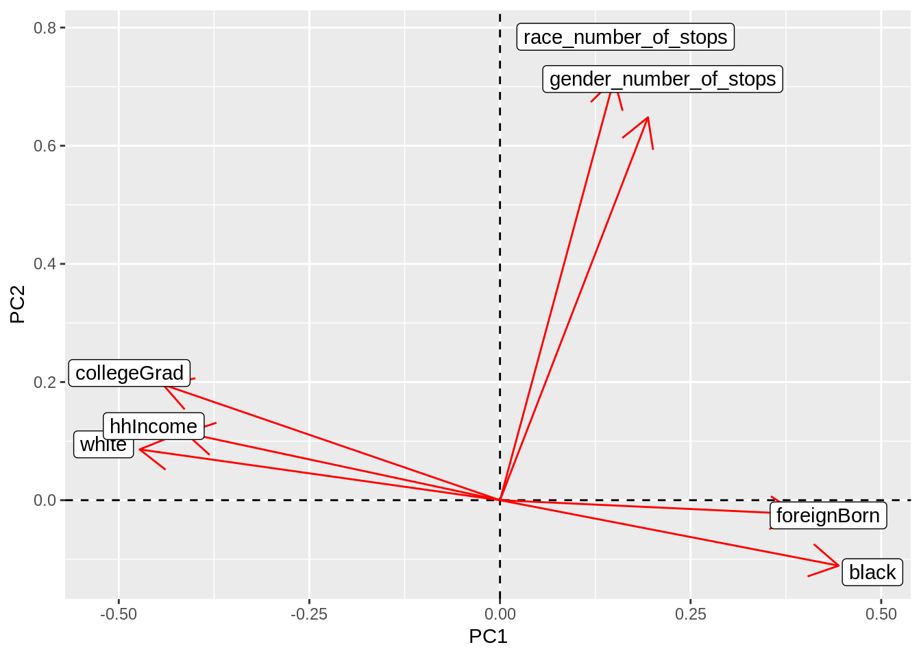
After principle component analysis was conducted and the plot was generated, many of my correlations found from before are further supported. We can see that PC1 separates those that have a college education, are white, and have a high household income from the number of stops by race and gender and those that are foreign born or black. Thus, this information supports my assertions that whites tend to be more college educated and have a higher household income in Minneapolis than those that are black or foreign born. Furthermore, whites are stopped at a lower rate than their non-white counterparts. One other interesting correlation is that both non-white men and women tend to be stopped at a higher rate than whites regardless of gender.